The tidyeval framework is a rather new, and in parts complementary, framework to dealing with non-standarde evaluation (NSE) in R. In short, NSE is about capturing some R-code, witholding execution, maybe editing the code, and finally execuing it later and/or somewhere else.
This post borrows heavily by Edwin Thon’s great post, and this post by the same author.
In addtion, most of the knowledge is derived from Hadley Wickham’s book Advanced R.
The typical base R culprits are eval(), and quote() or substitute(),
respectively.
library(tidyverse)  # load tidyeval too
library(rlang)  # more on tidyeval
library(pryr)  # working with environments
##
## Attaching package: 'pryr'
## The following object is masked from 'package:rlang':
##
##     bytes
## The following objects are masked from 'package:purrr':
##
##     compose, partial
What’s the difference between base nse and tidyeval nse?
And why should I bother?
Let’s look at some border case that show the difference quite strikingly.
Consider this base nse code:
base_NSE_fun <- function(some_arg) {
  some_var <- 10
  quote(some_var + some_arg)
}
base_NSE_fun(4) %>% eval()
## Error in eval(.): object 'some_var' not found
It does not work. eval() has no idea about the environment in which some_var is defined. (And in addition, quote() will take its arguments too literally, but we spare that for later.)
We might had expected the code above to work, however. That’s where tidyeval comes into play:
See here:
tidy_eval_fun <- function(some_arg) {
  some_var <- 10
  quo(some_var + some_arg)
}
tidy_eval_fun(4) %>% rlang::eval_tidy()
## [1] 14
Does work. With tidyeval, the environment of the variables are memorized. With base R, the environment is forgotton.
Looking at the chain of environments
What’s the enclosing environment of eval()? We can get hold of that environment using the function environment():
environment(eval)
## <environment: namespace:base>
What’s that for a strange environment? Well, that’s the NAMESPACE of package base, the exported objects of that package. A namespace is useful so the searchpath will not be cluttered by too many objects. Using a namespace we can define which objects should be made (easily) accessible to the users.
But in this environment, for sure, we will not have put some variable. How comes that this code does wor:
vanilla_x <- 1
eval(vanilla_x)
## [1] 1
What’s the environment of vanilla_x? We can access the enclosing environment of some object using this code:
pryr::where("vanilla_x")
## <environment: R_GlobalEnv>
So, if eval() looks in the namespace of base how comes that it finds some object in the global environment?
The answer is called lexical scoping. There’s a chain or ladder of enclosing environments, where the value is looked for. The total of this chaining is the search path.
Hadley Wickham illustrates this chain using this diagram in this chapter of Adv R:
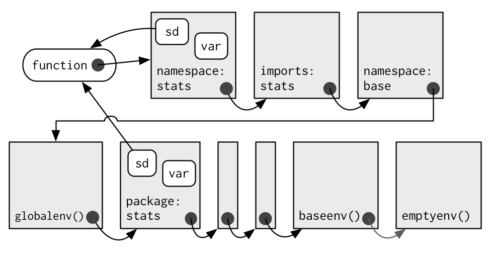
Each arrow coming from a grey dot refers to the enclosing environment of some object or function. The enclosing environment is the “home” environment, where the object was created.
We see that each object has an environment, and each environment has exactly one “parent” environment - with the notably execption of the emptyenv which is the first “ancestor” of this sequence.
Different types of environments
A function can and does have four environments:
- The enclosing environment: The environment where the fun was created; this environment is used for lexical scoping
- The executing environment: The environment where a fun is executed
- The binding environment: The environment(s) where some object is bound to the function
- The calling environment: The environment where the fun was called from
What substitute() can and cannot do
substitute() is the counterpart of quote() for use within functions. Do not use quote() within functions, use substitue() instead (or the tidyeval counterpart).
Consider:
base_eval_fun2 <- function(some_arg) {
  some_var <- 10
  substitute(some_var + some_arg)
}
base_eval_fun2(4) %>% rlang::eval_tidy()
## [1] 14
Great! Appears to work, does is not? Not exactly. Look what the function
call tidy_eval_fun2(4) is actually returning:
base_eval_fun2(4)
## 10 + 4
The result is quite hard coded (Thanks Edwin for pointing that out!). Compare the tidyeval variant:
tidy_eval_fun2 <- function(some_arg) {
  some_var <- 10
  quo(some_var + some_arg)
}
tidy_eval_fun2(4)
## <quosure: local>
## ~some_var + some_arg
Now we do not get the “hard” values but the variables AND their environment is carried over. We might change the expression or carry it to another environment where some_arg has some other value.