This posts shows data cleaning and preparation for a data set on a statistics test (NHST inference). Data is published under a CC-licence, see here.
Data was collected 2015 to 2017 in statistics courses at the FOM university in different places in Germany. Several colleagues helped to collect the data. Thanks a lot! Now let’s enjoy the outcome (and make it freely available to all).
Raw N is 743. The test consists of 40 items which are framed as propositions; students are asked to respond with either “true” or “false” to each item. In addition, self-rating of proportion correct, study time and interest in the subject are asked. Last column notes the number (proportion) of correct responses.
Raw data can be accessed here
df_raw <- read.csv("https://sebastiansauer.github.io/data/test_inf_raw.csv")
Alternatively, use this link: https://osf.io/zcvkd.
DOI of this data is: DOI 10.17605/OSF.IO/SJHUY, URL: https://osf.io/sjhuy
Some packages:
library(tidyverse)
To make the data set less clumsy, let’s replace variable names.
test_inf_names <- names(df_raw)
df <- df_raw
names(df) <- paste("V", 1:ncol(df_raw), sep = "_")

df <- rename(df, study_time = V_43, self_eval = V_44, interest = V_45)
The vector test_inf_names can now serve as a codebook; the variable names are stored there.
The correct answers for the 40 questions are:
correct <- c(
  T, T, T, T, F,
  F, F, F, F, T,
  T, T, F, T, T,
  T, T, T, T, F,
  F, T, T, F, T,
  F, F, F, T, F,
  T, T, F, T, T,
  F, T, T, T, F
)
We can now compare the actual answers to the correct ones for each respondent. Let’s leave that for later :-) What’s more, the items (questions) have changed over time. Malheuresement, the software used for delivering the survey (Google forms) does not save the history (and I did not really either, I admit). So I am not 100% sure whether the “solution vector” above is correct for each and every (older) respondent.
Instead, in the first step, let’s focus on the data where the solution is already provided for brevity. This information is stored in V_46 (Punkte). Let’s convert that string to a number.
library(readr)
library(stringr)
df$score <- str_sub(df$V_46, start = 1, end = 2)
df$score <- as.numeric(df$score)
Out of curiosity, let’s look at the distribution of the score.
ggplot(df, aes(x = score)) +
  geom_histogram()
#> `stat_bin()` using `bins = 30`. Pick better value with `binwidth`.
#> Warning: Removed 443 rows containing non-finite values (stat_bin).
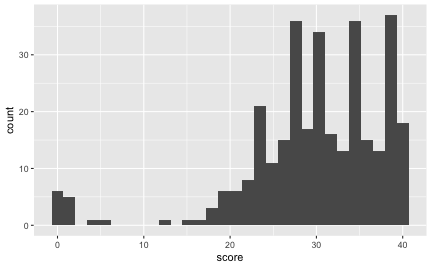
Note that the NAs are not shown. If a given student didn’t know anything, but would flip a coin for each answer, what’s the probability of getting x correct answers? In other words, in a sequence of 40 coin flips, what’s the probability of getting at least x right?
x <- 0:40
cdf <- pbinom(x, 40, prob = .5)

temp <- tibble(x, cdf)

ggplot() +
  geom_rect(aes(xmin = 15, xmax = 25, ymin = 0, ymax = 1), fill = "red", alpha = .3) +
  geom_line(data = temp, aes(x = x, y = cdf) )
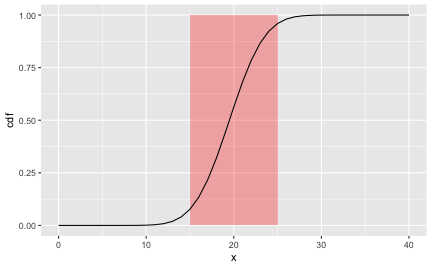
The diagram shows the probability of getting not more than x right. From a crude glance, say, 15 to 25 corrects answers are quite compatible with chance (coin tossing).
Let’s extract these and see how many cases are left.
df %>% filter(!is.na(score)) %>% nrow
#> [1] 321
df %>% filter(score > 16) %>% nrow
#> [1] 306
As the initial score variable was Punkte, let’s see how many NAs we had there.
df %>% filter(!is.na(V_46)) %>% nrow
#> [1] 764
OK, let’s assume all responses > 15 are “real” trials, not just guessing and clicking.
df <- filter(df, score > 15)
Association of study time and score
Now, what’s bothering me since years is whether (and how strong) there is an association between score and study time. Now finally, let’s jete a coup d’oeil.
r1 <- round(cor(df$study_time, df$score, use = "complete.obs"), 2)

p1 <- ggplot(df) +
  aes(x = study_time, y = score) +
  geom_jitter() + geom_smooth() +
  annotate(label = paste("r = ", r1), geom = "label", x = 4, y = 20, hjust = 0)

p1
#> `geom_smooth()` using method = 'loess' and formula 'y ~ x'
#> Warning: Removed 68 rows containing non-finite values (stat_smooth).
#> Warning in simpleLoess(y, x, w, span, degree = degree, parametric =
#> parametric, : pseudoinverse used at 3
#> Warning in simpleLoess(y, x, w, span, degree = degree, parametric =
#> parametric, : neighborhood radius 1
#> Warning in simpleLoess(y, x, w, span, degree = degree, parametric =
#> parametric, : reciprocal condition number 0
#> Warning in predLoess(object$y, object$x, newx = if
#> (is.null(newdata)) object$x else if (is.data.frame(newdata))
#> as.matrix(model.frame(delete.response(terms(object)), : pseudoinverse used
#> at 3
#> Warning in predLoess(object$y, object$x, newx = if
#> (is.null(newdata)) object$x else if (is.data.frame(newdata))
#> as.matrix(model.frame(delete.response(terms(object)), : neighborhood radius
#> 1
#> Warning in predLoess(object$y, object$x, newx = if
#> (is.null(newdata)) object$x else if (is.data.frame(newdata))
#> as.matrix(model.frame(delete.response(terms(object)), : reciprocal
#> condition number 0
#> Warning: Removed 68 rows containing missing values (geom_point).

library(ggExtra)
#ggMarginal(p1)
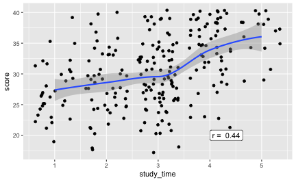
And the correlation is 0.441; hey, that’s quite strong!
Let’s also check ordinal correlation:
cor(df$study_time, df$score, method = "spearman", use = "complete.obs")
#> [1] 0.452
cor(df$study_time, df$score, method = "kendall", use = "complete.obs")
#> [1] 0.349
Given some measurement error, it can be speculated that the real, unattenuated correlation is quite substantial indeed.
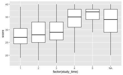
Maybe have a lookt at boxplots, as study time is not really metric:
ggplot(df) +
  aes(x = factor(study_time), y = score) +
  geom_boxplot()
Assocation of interest and score
Similarly, if one is interested in the subject, does she scores higher?
r2 <- round(cor(df$interest, df$score, use = "complete.obs"), 2)

p2 <- ggplot(df) +
  aes(x = interest, y = score) +
  geom_jitter() + geom_smooth() +
  annotate(label = paste("r = ", r2), geom = "label", x = 4, y = 20, hjust = 0)
p2
#> `geom_smooth()` using method = 'loess' and formula 'y ~ x'
#> Warning: Removed 68 rows containing non-finite values (stat_smooth).
#> Warning: Removed 68 rows containing missing values (geom_point).

#ggMarginal(p2)
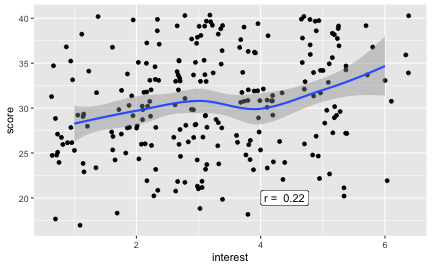
Weaker, but detectable.
Association of self-evaluation and score
Well, if I think I will score poorly (superb), will I do so? Does my self-image match the actual outcome?
r3 <- round(cor(df$self_eval, df$score, use = "complete.obs"), 2)

p3 <- ggplot(df) +
  aes(x = self_eval, y = score) +
  geom_jitter() + geom_smooth() +
  annotate(label = paste("r = ", r3), geom = "label", x = 8, y = 20, hjust = 0)
p3
#> `geom_smooth()` using method = 'loess' and formula 'y ~ x'
#> Warning: Removed 68 rows containing non-finite values (stat_smooth).
#> Warning: Removed 68 rows containing missing values (geom_point).

#ggMarginal(p3)
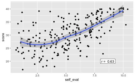
Oh, that’s strong; folks know when they’ll nail it. Good.
Correlation matrix
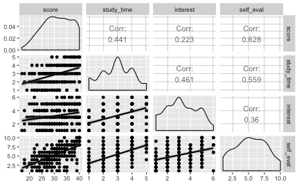
Finally, let’s look at the correlation matrix of the variables mentioned above.
library(corrr)

df %>%
  select(score, study_time, interest, self_eval) %>%
  correlate %>%
  shave   -> r_mat

r_mat
#> # A tibble: 4 × 5
#>      rowname score study_time interest self_eval
#>        <chr> <dbl>      <dbl>    <dbl>     <dbl>
#> 1      score    NA         NA       NA        NA
#> 2 study_time 0.441         NA       NA        NA
#> 3   interest 0.223      0.461       NA        NA
#> 4  self_eval 0.628      0.559     0.36        NA

corrr::rplot(r_mat)
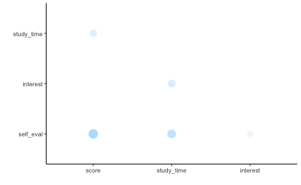
A scatter plot matrix can be of interest, too.
library(GGally)


df %>%
  select(score, study_time, interest, self_eval) %>%
  ggpairs(
    lower = list(
    continuous = "smooth",
    combo = "facetdensity"
  ))
#> Warning in (function (data, mapping, alignPercent = 0.6, method =
#> "pearson", : Removed 68 rows containing missing values
#> Warning in (function (data, mapping, alignPercent = 0.6, method =
#> "pearson", : Removed 68 rows containing missing values
#> Warning in (function (data, mapping, alignPercent = 0.6, method =
#> "pearson", : Removed 68 rows containing missing values
#> Warning: Removed 68 rows containing non-finite values (stat_smooth).
#> Warning: Removed 68 rows containing missing values (geom_point).
#> Warning: Removed 68 rows containing non-finite values (stat_density).
#> Warning in (function (data, mapping, alignPercent = 0.6, method =
#> "pearson", : Removed 68 rows containing missing values
#> Warning in (function (data, mapping, alignPercent = 0.6, method =
#> "pearson", : Removed 68 rows containing missing values
#> Warning: Removed 68 rows containing non-finite values (stat_smooth).
#> Warning: Removed 68 rows containing missing values (geom_point).
#> Warning: Removed 68 rows containing non-finite values (stat_smooth).
#> Warning: Removed 68 rows containing missing values (geom_point).
#> Warning: Removed 68 rows containing non-finite values (stat_density).
#> Warning in (function (data, mapping, alignPercent = 0.6, method =
#> "pearson", : Removed 68 rows containing missing values
#> Warning: Removed 68 rows containing non-finite values (stat_smooth).
#> Warning: Removed 68 rows containing missing values (geom_point).
#> Warning: Removed 68 rows containing non-finite values (stat_smooth).
#> Warning: Removed 68 rows containing missing values (geom_point).
#> Warning: Removed 68 rows containing non-finite values (stat_smooth).
#> Warning: Removed 68 rows containing missing values (geom_point).
#> Warning: Removed 68 rows containing non-finite values (stat_density).
Debrief
As a teacher, I feel reassured that study time is associated with test performance.
Processed data can also be downloaded, here.